
Get the most out of your categorical features and improve model performance with Embedding Encoder
Dealing with categorical features
For a number of reasons categorical features often require special treatment in the context of machine learning models.
First, most algorithms are not built to work with non-numeric features, which rules out any strings in your dataset.
Second, there is often no obvious relationship between different classes of a categorical variable. How do “red”, “blue” and “green” compare to each other? Even in the context of ordinal categorical features, where there is a clear ordering or classes, it is generally not possible to define how “different” they are; we know Monday always comes before Tuesday and after Sunday, so they are ordered, but they are not easily compared.
The way we were taught to deal with these situations is to one-hot encode the variable, so that each class becomes its own feature of 1s and 0s. However, with high cardinality features with a lot of unique values, one-hot encoding can lead to very sparse datasets, making it computationally inefficient to train models.
The latter is a common challenge in natural language processing, because each word would get its own dummy variable.
Using embeddings outside of the field of natural language processing
Word embeddings is one of the most used techniques in the field of natural language processing (NLP). It consists on building trainable lookup tables that map words to numerical representations. This boosts the performance of the model compared to a simple frequency approach (i.e. counting how many times each word appears in the corpus) because embeddings retain the similarity between words in a chain of text. For example, the embedding representation of words such as “joy”, “happy” or “fun” oftentimes are very close.
While embeddings make the most sense in an unstructured text modeling environment, structured datasets with high cardinality categorical features can benefit from a very similar technique called entity embedding, where each class of a categorical feature is mapped to a vector representation, leading to dense datasets that retain information about the similarity of the classes. This technique was popularized after the team that landed in the 3rd place of the Rossmann Kaggle competition used it.
Although Python implementations of this approach have surfaced over the years, we are not aware of any library that integrates this functionality into scikit-learn, so we built it.
Enter Embedding Encoder!
![]()
Embedding Encoder is a scikit-learn-compliant transformer that converts categorical variables into numeric vector representations. This is achieved by creating a small multilayer perceptron architecture in which each categorical variable is passed through an embedding layer, for which weights are extracted and turned into DataFrame columns.
We will go through the code in a notebook created to showcase the usefulness of the library that builds a model for the Rossman Store Sales dataset from Kaggle, by using it to process high cardinality categorical columns . Then, we compare the performance of this approach to an alternative in which high cardinality features are transformed with scikit-learn’s Ordinal Encoder.
Let’s get to work
Since this is just a demo of the capabilities of Embedding Encoder we will just perform very basic data processing on the dataset by just filling null values and removing columns with a very high percentage of null values.
Do not forget to install Embedding Encoder from PyPI!
pip install embedding-encoder[full]
Data preparation
import pandas as pd
import numpy as np
from sklearn.compose import ColumnTransformer
from sklearn.preprocessing import OneHotEncoder, StandardScaler, OrdinalEncoder
from sklearn.pipeline import make_pipeline
from sklearn.model_selection import train_test_split
from sklearn.impute import SimpleImputer
from sklearn.ensemble import RandomForestRegressor
from sklearn.metrics import mean_squared_error, mean_absolute_percentage_error

from embedding_encoder import EmbeddingEncoder
from embedding_encoder.utils.compose import ColumnTransformerWithNames
store_df = pd.read_csv("store.csv")
train_df = pd.read_csv("train.csv", dtype={"StateHoliday": str})

df = train_df.merge(store_df, how="left", left_on=train_df.Store, right_on=store_df.Store)
df.drop(["key_0", "Store_y"], axis=1, inplace=True)
df = df.rename(columns={"Store_x":"Store"})

df.drop(["Promo2SinceWeek", "Promo2SinceYear", "PromoInterval"], axis=1, inplace=True)
df = df.sample(frac=0.2) # We sample 20% of the dataset, about 200k rows, to speed up training
X = df.drop(["Sales", "Date"], axis=1)
y = df["Sales"]

X_train, X_test, y_train, y_test = train_test_split(X, y, test_size=0.2)
Now we have our data split into train and test sets and we can use a pipeline for processing. Since Embedding Encoder is scikit-learn compliant it can be used in a pipeline together with other data processing libraries.
But before building a pipeline, we have to create three lists of columns to use the encoders on them. The first list will be for categorical columns with very high cardinality, the second list will have categorical columns with low cardinality and the third list will be a list of numerical columns to process.
categorical_high = ["Store", "CompetitionOpenSinceYear", "CompetitionOpenSinceMonth", "DayOfWeek"]
categorical_low = ["Open", "Promo", "SchoolHoliday", "Promo2", "StateHoliday", "StoreType", "Assortment"]
numeric = ["Customers", "CompetitionDistance"]
Now we can start building our pipelines to compare. We can easily create a function to build them and use a parameter to differentiate the Embedding Encoder from the Ordinal Encoder one.
def build_pipeline(mode: str):
    if mode == "embeddings":
        high_cardinality_encoder = EmbeddingEncoder(task="regression")
    else:
        high_cardinality_encoder= OrdinalEncoder()
        one_hot_encoder = OneHotEncoder(handle_unknown="ignore")
        scaler = StandardScaler()
        imputer = ColumnTransformerWithNames([("numeric", SimpleImputer(strategy="mean"), numeric),
                                              ("categorical", SimpleImputer(strategy="most_frequent"),
                                               categorical_low+categorical_high)])
        processor = ColumnTransformer([("one_hot", one_hot_encoder, categorical_low),
                                       (mode, high_cardinality_encoder, categorical_high),
                                       ("scale", scaler, numeric)])
    return make_pipeline(imputer, processor, RandomForestRegressor())

embeddings_pipeline = build_pipeline("embeddings")
ordinal_pipeline = build_pipeline("ordinal")
With the pipelines ready now we just need to fit, predict and compare results. Since this is a regression task (sales value), we will use mean squared error and mean absolute percentage error for model evaluation.
embeddings_pipeline.fit(X_train, y_train)
embedding_preds = embeddings_pipeline.predict(X_test)

ordinal_pipeline.fit(X_train, y_train)
ordinal_preds = ordinal_pipeline.predict(X_test)
When we calculate and print these metrics, we get the following results:
Model using Ordinal Encoder:
Root Mean Squared Error: 579.9272913513555
Model using Embedding Encoder:
Root Mean Squared Error: 554.4734797807192
Et voila! Embedding Encoder performed marginally better than ordinal encoder, albeit the pipeline that uses embeddings takes more time to run. The interesting thing about this is the fact that this is the tip of the iceberg in terms of improving the performance of the model and Embedding Encoder is a tool with lots of capabilities.
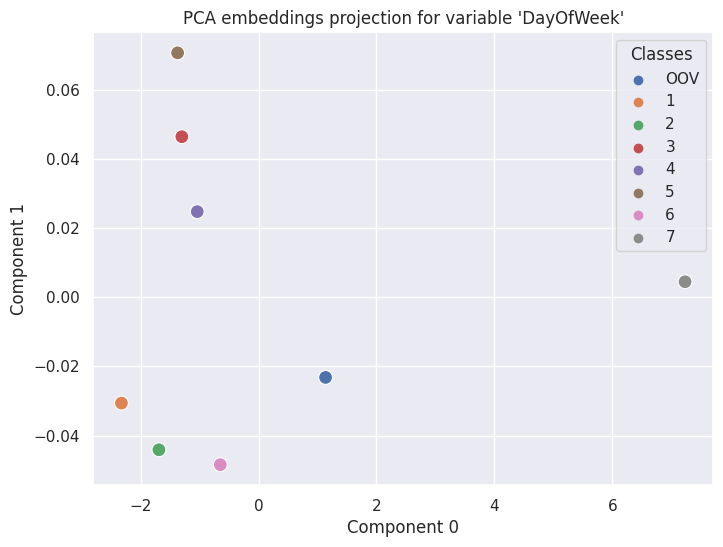
The generated embeddings can be plotted in a 2D space in order to understand whether the encoder could extract actual value from the categorical features. This requires seaborn, which can be easily installed separately or by using the [full] or [sns] parameters in pip install for Embedding Encoder.
Customizing embedding encoder
Numeric features can be included as an additional input to the neural network by passing the numerical columns list as a parameter to the encoder, which can lead to better results depending on the dataset you are working with.
The network architecture can be modified to include more layers, wider layers, and different dropout rates, and the training loop can have its batch size and epochs customized as well.
Non-Tensorflow usage
Tensorflow can be tricky to install on some systems, which could make Embedding Encoder less appealing if the user has no intention of using TF for modeling.
There are actually two partial ways of using Embedding Encoder without a TF installation.
Because TF is only used and imported in the EmbeddingEncoder.fit() method, once EE or the pipeline that contains EE has been fit, TF can be safely uninstalled; calls to methods like EmbeddingEncoder.transform() or Pipeline.predict() should raise no errors.
Embedding Encoder can save the mapping from categorical variables to embeddings to a JSON file which can be later imported by setting pretrained=True, requiring no TF whatsoever. This also opens up the opportunity to train embeddings for common categorical variables on common tasks and saving them for use in downstream tasks.
Installing EE without Tensorflow is as easy as removing “[tf]” from the install command.
Final remarks
Embedding Encoder is just another tool in the toolkit, although a very cool and potent one, but at the end of the day it falls on you to understand the situation and the data you are working with in order to get the most out of it.
If you want to know more about the features of Embedding Encoder, feel free to check our Github repository. There you will find more explanations on how to use the tool and who knows… maybe you will find more interesting results or even win a machine learning competition by using this.